Units and Conventions

Fourier transform conventions

We follow the (reasonably standard) conventions of the Fourier transform (e.g., Bracewell’s “system 1”).

Forward transform:

\[ F(s) = \int_{-\infty}^\infty f(x) e^{-i 2 \pi x s} \mathrm{d}x \]

Inverse transform:

\[ f(x) = \int_{-\infty}^\infty F(s) e^{i 2 \pi x s} \mathrm{d}s \]

Baseline Convention

For two antennas ant1 and ant2, the baseline convention describes how the baseline between them is represented in UVW coordinates and whether the positive baseline is measured from ant1->ant2, or from ant2->ant1. MPoL follows the former, standard baseline convention as laid out in Thompson, Moran, and Swenson and other radio interferometry textbooks. However, CASA follows a historically complicated convention described in CASA Memo 2. The difference between the two can be expressed as the complex conjugate of the visibilities. So, if you find that your image appears upside down and mirrored, you’ll want to take np.conj of your visibilities before proceeding.

Continuous representation of interferometry

Consider some astronomical source parameterized by its sky brightness distribution \(I\). The sky brightness is a function of position on the sky. For small fields of view (typical to single-pointing ALMA or VLA observations) we parameterize the sky direction using the direction cosines \(l\) and \(m\), which correspond to R.A. and Dec, respectively. In that case, we would have a function \(I(l,m)\). The sky brightness is an intensity, so it has units of \(\mathrm{Jy\,arcsec}^{-2}\) (equivalently \(\mathrm{Jy\, beam}^{-1}\), where \(\mathrm{beam}\) is the effective area of the synthesized beam).

The real domain is linked to the Fourier domain, also called the visibility domain, via the Fourier transform

\[ {\cal V}(u,v) = \int \int I(l,m) \exp \left \{- 2 \pi i (ul + vm) \right \} \, \mathrm{d}l\,\mathrm{d}m. \]

This integral demonstrates that the units of visibility function (and samples of it) are \(\mathrm{Jy}\).

Note

This simplified relationship omits many additional effects that modify the cosmic intensity before it is recorded as visibility data. A full treatment of these effects can be mathematically described by the Radio Interferometric Measurement Equation (RIME). See the Revisiting the radio interferometer measurement equation series by O. Smirnov, 2011 for more details.

Discretized representation

There are several annoying pitfalls that can arise when dealing with discretized images and Fourier transforms, and most relate back to confusing or ill-specified conventions. The purpose of this page is to explicitly define the conventions used throughout MPoL and make clear how each transformation relates back to the continuous equations.

Pixel fluxes and Cube dimensions

• Throughout the codebase, any sky plane cube representing the sky plane is assumed to have units of \(\mathrm{Jy\,arcsec}^{-2}\).

• The image cubes are packed as 3D arrays (nchan, npix, npix).

• The “rows” of the image cube (axis=1) correspond to the \(m\) or Dec axis. There are \(M\) number of pixels in the Dec axis.

• The “columns” of the image cube (axis=2) correspond to the \(l\) or R.A. axis. There are \(L\) number of pixels in the R.A. axis.

Angular units

For nearly all user-facing routines, the angular axes (the direction cosines \(l\) and \(m\) corresponding to R.A. and Dec, respectively) are expected to have units of arcseconds. The sample rate of the image cube is set via the cell_size parameter, in units of arcsec. Internally, these quantities are represented in radians. Let the pixel spacing be represented by \(\Delta l\) and \(\Delta m\), respectively.

Fourier units

The sampling rate in the Fourier domain is inversely related to the number of samples and the sampling rate in the image domain. I.e., the grid spacing is

\[\begin{split} \Delta u = \frac{1}{L \Delta l} \\ \Delta v = \frac{1}{M \Delta m}. \end{split}\]

If \(\Delta l\) and \(\Delta m\) are in units of radians, then \(\Delta u\) and \(\Delta v\) are in units of cycles per radian. Thanks to the geometric relationship of the interferometer, the spatial frequency units can equivalently be expressed as the baseline lengths measured in multiples of the observing wavelength \(\lambda\).

For example, take an observation with ALMA band 6 at an observing frequency of 230 GHz, corresponding to a wavelength of 1.3mm. A 100 meter baseline between antennas will measure a spatial frequency of \(\frac{100\,\mathrm{m} }{ 1.3 \times 10^{-3}\,\mathrm{m}} \approx 77 \mathrm{k}\lambda\) or 77,000 cycles per radian.

For more information on the relationship between baselines and spatial frequencies, see TMS Eqn Chapter 2.3, equations 2.13 and 2.14. Internally, MPoL usually represents spatial frequencies in units of \(\mathrm{k}\lambda\).

For reference, here are some typical ALMA baseline lengths and their (approximate) corresponding spatial frequencies at common observing frequencies

baseline	100 GHz (Band 3)	230 GHz (Band 6)	340 GHz (Band 7)
10 m	3 \(\mathrm{k}\lambda\)	8 \(\mathrm{k}\lambda\)	11 \(\mathrm{k}\lambda\)
50 m	17 \(\mathrm{k}\lambda\)	38 \(\mathrm{k}\lambda\)	57 \(\mathrm{k}\lambda\)
100 m	33 \(\mathrm{k}\lambda\)	77 \(\mathrm{k}\lambda\)	113 \(\mathrm{k}\lambda\)
500 m	167 \(\mathrm{k}\lambda\)	384 \(\mathrm{k}\lambda\)	567 \(\mathrm{k}\lambda\)
1 km	334 \(\mathrm{k}\lambda\)	767 \(\mathrm{k}\lambda\)	1 \(\mathrm{M}\lambda\)
5 km	2 \(\mathrm{M}\lambda\)	4 \(\mathrm{M}\lambda\)	6 \(\mathrm{M}\lambda\)
10 km	3 \(\mathrm{M}\lambda\)	8 \(\mathrm{M}\lambda\)	11 \(\mathrm{M}\lambda\)
16 km	5 \(\mathrm{M}\lambda\)	12 \(\mathrm{M}\lambda\)	18 \(\mathrm{M}\lambda\)

Occasionally, it is useful to represent the cartesian Fourier coordinates \(u\), \(v\) in polar coordinates \(q\), \(\phi\)

\[\begin{split} q = \sqrt{u^2 + v^2}\\ \phi = \mathrm{atan2}(v,u). \end{split}\]

\(\phi\) represents the angle between the \(+u\) axis and the ray drawn from the origin to the point \((u,v)\). Following the numerical conventions of the arctan2 function, \(\phi\) is defined over the range \((-\pi, \pi]\).

The discrete Fourier transform

Since we are dealing with discrete quantities (pixels), we use the discrete versions of the Fourier transform (DFT), carried out by the Fast Fourier transform (FFT). Throughout the package we use the implementations in numpy or PyTorch: they are mathematically the same, but PyTorch provides the opportunities for autodifferentiation. For both the forward and inverse transforms, we assume that norm='backward', the default setting. This means we don’t need to keep account for the \(L\) or \(M\) prefactors for the forward transform, but we do need to account for the \(U\) and \(V\) prefactors in the inverse transform.

Forward transform: As before, we use the forward transform to go from the image plane (sky brightness distribution) to the Fourier plane (visibility function). This is the most common transform used in MPoL because RML can be thought of as a type of forward modeling procedure: we’re proposing an image and carrying it to the visibility plane to check its fit with the data. In numpy, the forward FFT is defined as

\[ \mathtt{FFT}(I_{l,m}) = \sum_{l=0}^{L-1} \sum_{m=0}^{M-1} I_{l,m} \exp \left \{- 2 \pi i (ul/L + vm/M) \right \} \]

To make the FFT output an appropriate representation of the continuous forward Fourier transform, we need to account for the spacing of the input samples. The FFT knows only that it was served a sequence of numbers, it does not know that the samples in \(I_{l,m}\) are spaced cell_size apart. To do this, we just need to account for the spacing as a prefactor (i.e., converting the \(\mathrm{d}l\) to \(\Delta l\)), following TMS Eqn A8.18

\[ V_{u,v} = (\Delta l)(\Delta m) \mathtt{FFT}(I_{l,m}) \]

In this context, the \(u,v\) subscripts indicate the elements of the \(V\) array. As long as \(I_{l,m}\) is in units of \(\mathrm{Jy} / (\Delta l \Delta m)\), then \(V\) will be in the correct output units (flux, or Jy).

Inverse transform: The inverse transform is used within MPoL to produce a quick diagnostic image from the visibilities (called the “dirty image”). As you might expect, this is the inverse operation of the forward transform. Numpy and PyTorch define the inverse transform as

\[ \mathtt{iFFT}({\cal V}_{u,v}) = \frac{1}{U} \frac{1}{V} \sum_{l=0}^{U-1} \sum_{m=0}^{V-1} {\cal V}_{u,v} \exp \left \{2 \pi i (ul/L + vm/M) \right \} \]

If we had a fully sampled grid of \({\cal V}_{u,v}\) values, then the operation we’d want to carry out to produce an image needs to correct for both the cell spacing and the counting terms

\[ I_{l,m} = U V (\Delta u)(\Delta v) \mathtt{iFFT}({\cal V}_{u,v}) \]

For more information on this procedure as implmented in MPoL, see the Gridder class and the source code of its get_dirty_image() method. When the grid of \({\cal V}_{u,v}\) values is not fully sampled (as in any real-world interferometric observation), there are many subtleties beyond this simple equation that warrant consideration when synthesizing an image via inverse Fourier transform. For more information, consult the seminal Ph.D. thesis of Daniel Briggs.

Image Cube Packing for FFTs

Numerical FFT routines expect that the first element of an input array (i.e., array[i,0,0]) corresponds to the zeroth spatial (\(l,m\)) or frequency (\(u,v\)) coordinate. This convention is quite different than the way we normally look at images. As described above, MPoL deals with three dimensional image cubes of shape (nchan, npix, npix), where the “rows” of the image cube (axis=1) correspond to the \(m\) or Dec axis, and the “columns” of the image cube (axis=2) correspond to the \(l\) or R.A. axis. Normally, the zeroth spatial component \((l,m) = (0,0)\) is in the center of the array (at position array[i,M/2,L/2]), so that when an array is visualized (say with matplotlib.pyplot.imshow, origin="lower"), the center of the array appears in the center of the image.

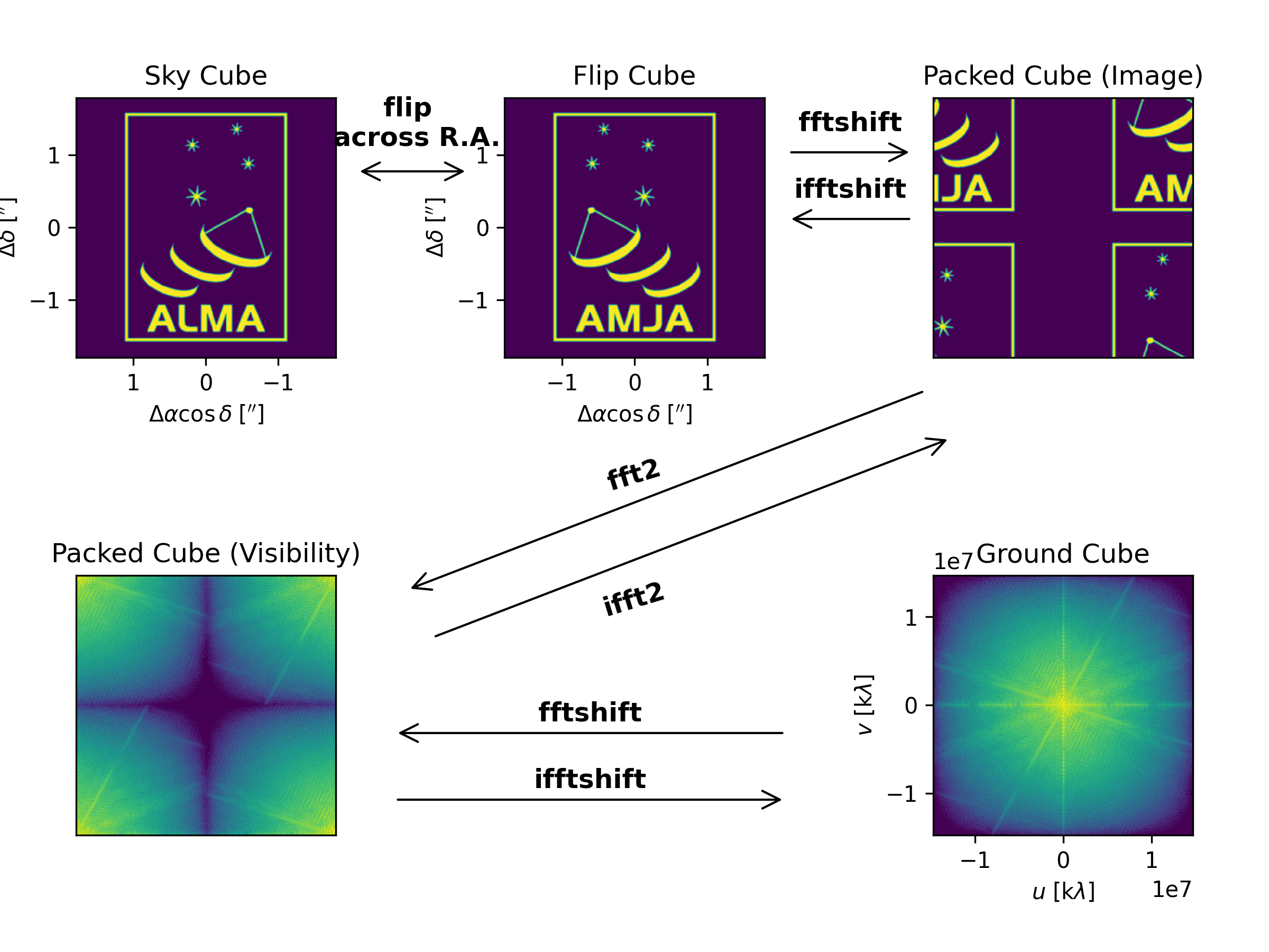
Complicating this already non-standard situation is the fact that astronomers usually plot images as seen on the sky: with north (\(m\)) up and east (\(l\)) to the left. Throughout the MPoL base, we call these cubes ‘sky cubes,’ see the above figure for a representation. In order to display sky cubes properly with routines like matplotilb.pyplot.imshow, when indexed as array[i,j,k], an increasing k index must correspond to decreasing values of \(l\). (It’s OK that an increasing j index corresponds to increasing values of \(m\), however we must be certain to include the origin="lower argument when using matplotlib.pyplot.imshow).

Correctly taking the Fourier transform of a sky cube requires several steps. First, we must flip the cube across the R.A. axis (axis=2) to create an array[i,j,k] which has both increasing values of j and k correspond to increasing values of \(m\) and \(l\), respectively. We call this intermediate product a ‘flip cube.’

Then, the cube must be packed such that the first element(s) of an input array (i.e., array[i,0,0]) correspond to the zeroth spatial coordinates \((l,m) = (0,0)\). Thankfully, we can carry out this operation easily using fftshift functions commonly provided by FFT packages like numpy.fft or torch.fft. We shift across the Dec and R.A. axes (axis=1 and axis=2) leaving the channel axis (axis=0) untouched to create a ‘packed image cube.’ MPoL has convenience functions to carry out both the flip and packing operations called mpol.utils.sky_cube_to_packed_cube() and the inverse process mpol.utils.packed_cube_to_sky_cube().

After the FFT is correctly applied to the R.A. and Dec dimensions using fft2, the output is a packed visibility cube, where the first elements (i.e., array[i,0,0]) correspond to the zeroth spatial frequency coordinates \((u,v) = (0,0)\). To translate this cube back into something that’s more recognizable when plotted, we can apply the ifftshift operation along the \(v\) and \(u\) axes (axis=1 and axis=2) leaving the channel axis (axis=0) untouched to create a ‘ground visibility cube’. We choose to orient the visibility plane from the perspective of an areial observer looking down at an interferometric array on the ground, such that north is up and east is to the right, therefore no additional flip is required for the visibility cube. MPoL has convenience functions to carry out the unpacking operation mpol.utils.packed_cube_to_ground_cube() and the inverse process mpol.utils.ground_cube_to_packed_cube().

In practice, fftshift and ifftshift routines operate identically for arrays with an even number of elements (currently required by MPoL).